De novo footprint detection#
Overview#
Footprint-tools implements a footprint detection algorithm that simulates expected cleavage rates using a 6-mer DNase I cleavage preference model combined with density smoothing. Statistical significance of per-nucleotide cleavages are computed from a series emperically fit negative binomial distributions.
The process of calling footprints involves the following steps:
Computing expected cleavage counts and learning the dispersion (variance) model used to assign statistical significance to the observed per-nucleotide cleavage ratese
Statistical testing of observed vs. expected cleavages per-nucleotide
Combining adjacent p-values
Adjusting p-values for multiple testing by resampling
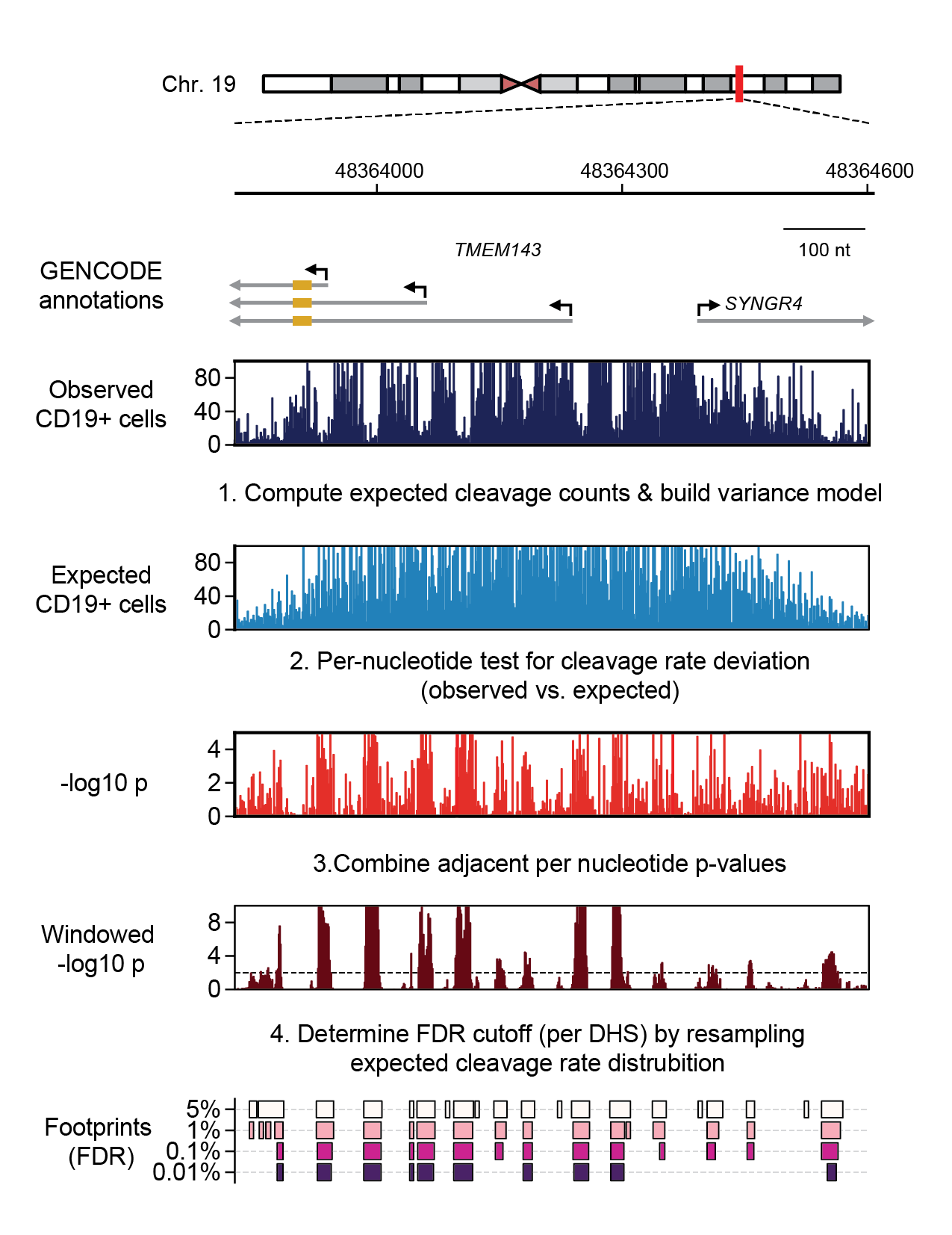
Example of de novo footprint detection at the TMEM143 promoter in CD19+ B cells.#
The above steps are performed by scripts installed as part of the footprint-tools python package.
Please see our manuscript for further details.
Computing expected cleavages#
We use a hierarchical approach to model the expected cleavages. First, for each base we compute the total cleavages within a small window (typically +/-5nt, total 11nt). We then smooth these values by computing the trimmed mean within a larger window. These values thus reflect both the local density of DNaseI cleavage (in 11 bp windows) and also the shape and magnitude of the entire DHS itself.
Building a dispersion model#
Because the vast majority of nucleotides are unoccupied on the genome, we can safely assume that most cleavages represent “background”. We take advantage of this to directly estimate the the variance in the observed cleavage counts at expected cleavage rates. To do this, we collect all nucleotides for a given expected cleavage rate (\(n=1,2,3,4,..\)) and fit a negative binomial to the distribution of observed cleavage counts (rates) at these nucleotides. Testing whether the observed cleavage at an individual nucleotide significantly deviates from expected is straightforward, we just use the negative binomial distribution for the expected cleavage count (at an idividual nucleotide) and compute the probability of the observed cleavage count (i.e., cumulative lower-tail probability).
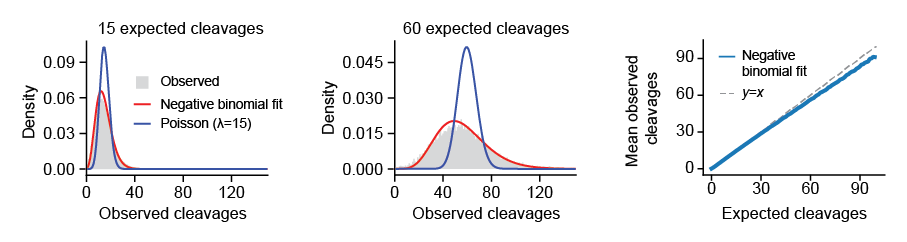
Example dispersion model. Left and middle, histogram of observed cleavages counts at nucleotides with 15 (left) and 60 (middle) expected cleavages. Red, maximum likelihood fit of negative binomial distribution. Blue, Poisson distribution with \(\lambda\) set to 15 or 60. Right, mean of observed cleavages vs. expected cleavages.#
Step-by-step guide#
Step 1: Align sequenced DNase I cleavages#
footprint-tools requires an alignment file in BAM format which can be made using any sequence alignment tool. The software uses all reads with a MAPQ > 0. Typically, we also mark tags as QC fail. Inclusion/exclusion of reads by MAPQ and other SAM flags can be specified during execution of the software.
Step 2: Create an index of the reference genome FASTA file#
The software uses an indexed FASTA file to enable rapid lookups of genomic sequences utilized by the sequence bias model. A FASTA file can be indexed using samtools.
samtools faidx /home/jvierstra/data/genomes/hg19/hg.ribo.all.fa
Step 3a: Download or create a 6-mer cleavage bias model#
The sequence bias model is the basis of footprint detection. A model file contains 2 columns that contain a sequence k-mer and a relative preference value. While the bias model can be of any k-mer size, DNase I sequence preference is best modeled using 6mers, with the cleavage occurring between the 3rd and 4th base.
You can download a pre-computed preference model for the human genome.
ACTTGC	0.222146731451
ACTTAC	0.215317065202
TCTTGC	0.208412818813
AAAATT	0.000316910682485
CAGATT	0.000311015040584
CAAATT	0.000310636101587
Note
The model provided in the repository was generated using UCSC genome build hg19. There should be not be a problem using this model for footprint detection in hg38.
Step 3b: Create a sequence preference model#
You can create your own sequence preference model using a
a provided template script.
The script counts the 6mer context of all the cleavage/insertional events
such that the 5’ end of the tags is in position 3’ nnn-Nnn 5’ end of read oriented for
strand mappped) and then compares it to the prevalence of that 6mer in
the mappable genome. As such, prerequisites for creating a bias model
are:
A BAM file from a naked DNaseI experiment
A genome mappability file corresponding to the read length of the reads in the BAM file (see below), and
An indexed FASTA file for the genome your BAM file refers to.
./generate_bias_model.sh --temporary-dir /tmp/jvierstra \
  reads.filtered.bam mappability.stranded.bed  \
  /home/jvierstra/data/genomes/hg19/hg.ribo.all.fa \
  naked.model.txt
The mappability file specifies the regions of the genome where the sequencing strategy can detect cleavage events. Fortunately, the ENCODE project (Roderic Guigo’s lab at CRG Barcelona) has created a track that predicts the alignability of positions by putative read length. The script above requires a file which contains regions where the 5’ positions are mappable in a stranded fashion. It is simple to convert the CRG track into a stranded mappability track:
# Creates a stranded mappability file for 36mer read length

wget http://hgdownload.cse.ucsc.edu/goldenpath/hg19/encodeDCC/wgEncodeMapability/wgEncodeCrgMapabilityAlign36mer.bigWig

bigWigToBedGraph wgEncodeCrgMapabilityAlign36mer.bigWig /dev/stdout
| awk -v OFS="\t" '
        $4 >= 0.5 { print $1, $2, $3, ".", ".", "+";
        print $1, $2+36-1, $3+36-1, ".", ".", "-"; }
    '
| sort-bed --max-mem 16G -
> mappability.stranded.bed
Step 4: Create a dispersion model#
We use a negative binomial to compute the significance of per-nucleotide cleavage devations from the expected. The negative binomial has two parameters, mu and r. The command command_learn_dm emperically fits \(\mu\) and \(r\) from the observed cleavage data and then interpolates all values using linear regression. command_learn_dm writes a dispersion model in JSON format to standard out which can then be used with all follow-on analyses.
ftd learn_dm \
  --bias_model_file vierstra_el_al.6-mer.model.txt \
  intervals.bed reads.bam genome.fa
Note
An important step in footprint detection is inspection of the learned dispersion model. A poorly fit model will impair sensitivity.
The command_plot_dm command will plot diagnostic plots.
ftd plot_dm dm.json --histograms 5,50,100
In addition to the command-line interface, you can perform plotting directly with the Python packge. See the here for an example of how to visualize the dispersion model using python and matplotlib
Step 5: Compute per-nucleotide expected cleavages#
The command command_detect is used to compute per-nucleotide cleavages statistics:
ftd detect \
  --bias_model_file vierstra_et_al.6-mer.model.txt \
  --dispersion_model_file dm.json \
  intervals.bed reads.bam genome.fa
Example output:
The primary output of command_detect is a bedGraph file containing the per-nucleotide cleavage statistics for regions in the input file.
 # generated by footprint_tools version 1.3.0
 # chrom start   end     name    exp     obs     -log(pval)      -log(winpval)   fdr
 chr1    180800  180801  0.0000  0.0000  0.2658  -0.0000 1.0000
 chr1    180801  180802  0.0000  0.0000  0.2658  -0.0000 1.0000
 chr1    180802  180803  0.0000  0.0000  0.2658  -0.0000 1.0000
 chr1    180803  180804  0.0000  0.0000  0.2658  0.0275  0.1556
By default, footprints at outputed to BED-format files. One can use
the option --write_footprints to specify FDR thresholds used to
delineate footprints.
# generated by footprint_tools version 1.3.0
# thresholded @ FDR 0.01
# chrom start   end     name    name    fdr
chr1    180843  180854  .       0.0096
chr1    180864  180870  .       0.0096
chr1    181421  181438  .       0.0002
chr1    181445  181450  .       0.0031
Step 6: Retrieving footprints#
Footprints can be retrieved by thresholding on either p-values or the emperical FDR and then merging consecutive bases.
cat per-nucleotide.bedgraph \
    | awk -v OFS="\t" -v thresh=0.01 '$8 <= thresh { print $1, $2-3, $3+3; }' \
    | sort-bed --max-mem 8G - \
    | bedops -m - \
> ${output_dir}/interval.all.fps.\${thresh}.bed