Remote access and plotting posterior footprint probabilities

This notebook shows an example of how to access remotely hosted DGF data and generate a portion of Fig. 1b from Vierstra et al. 2020.

The plotting performed in this example relies on the python package genome-tools, which provides an assortment of ways to plot genomic data. You can find a short tutorial in the form of a python notebook here on the various features.

import matplotlib.pyplot as plt
import matplotlib.gridspec as gridspec

import pandas as pd
import numpy as np
import pysam

from genome_tools import genomic_interval
from genome_tools.plotting import gencode_annotation_track
from genome_tools.plotting import segment_track

def unpack(s):
    """Converts a 1-based UCSC coordinate string
    into a a genomic_interval object"""

    tmp = s.replace(",", "")
    (chrom, pos_str) = tmp.split(":")
    start, end = pos_str.split("-")
    return genomic_interval(chrom, int(start)-1, int(end))

class tabix_reader(object):
    def __init__(self, fname, interval):
        self.tabix_handle=pysam.TabixFile(fname)
        self.iter = self.tabix_handle.fetch(interval.chrom, interval.start, interval.end)
    def read(self, n=0):
        try:
            return next(self.iter) + "\n"
        except StopIteration:
            return ''
    def __iter__(self):
        return self
    def __next__(self):
        return self.read()

def tabix_query(filename, interval, fill_val=np.nan):
    """Call tabix and generate an array of strings for each line it returns.
       Posterior matrix removes positions where no sample has posterior value
       >0.8 to save space, so the function adds these positions back and fills them
       with a user-defined fill value
    """
    ret=pd.read_csv(
        tabix_reader(filename, interval),
        delimiter="\t", header=None,
        index_col=1).drop([0, 2], axis=1)

    ret.index.name="pos"
    ret.columns=np.arange(ret.shape[1])

    pos_index=pd.Index(np.arange(interval.start, interval.end))

    na_pos=pos_index[~pos_index.isin(ret.index)]
    na_df=pd.DataFrame(np.full([na_pos.shape[0], ret.shape[1]], fill_val), index=na_pos)

    return pd.concat([ret, na_df]).sort_index().T

Read in sample metadata

Read the sample metadata into a dataframe from Supplementary Table 1.

sample_info_file="https://resources.altius.org/~jvierstra/projects/footprinting.2020/Supplementary_Table_1.xlsx"
samples=pd.read_excel(sample_info_file, skiprows=16, index_col=0)
samples.head()

	Taxonomy_class	Taxonomy_system	Description	Individual ID	SPOT	Total_reads	Unique_reads	DCC_experiment_id	DCC_library_id	DCC_biosample_id	DCC_file_id_FDR_1%
Identifier
AG10803-DS12374	Primary	Connective	Abdominal skin Fibroblast	Z68	0.6904	369891377	220628368	ENCSR000EMB	ENCLB410ZZZ	ENCBS287ITL	ENCFF989WCF
AoAF-DS13513	Primary	Connective	Aortic Adventitial Fibroblasts	Z94	0.6395	393665970	317762220	ENCSR000EMC	ENCLB412ZZZ	ENCBS408ZNY	ENCFF587TUM
CD19+-DS17186	Primary	Hematopoietic	CD19+ B cells	Z8	0.5056	601010994	488593380	ENCSR381PXW	ENCLB800FZO	ENCBS469TSJ	ENCFF976ZIX
CD20+-DS18208	Primary	Hematopoietic	B cells	Z144	0.5570	300895833	229005077	ENCSR000EMJ	ENCLB425ZZZ	ENCBS483ENC	ENCFF197KBO
GM06990-DS7748	Lines	Hematopoietic	Lymphoblastoid	Z73	0.6547	238189351	142211228	ENCSR000EMQ	ENCLB435ZZZ	ENCBS057ENC	ENCFF825VXW

Define region to plot

The code below opens up the remotely hosted TABIX file and pulls the data for a specified region.

If you get an OSError: could not open index for... try deleting the .tbi file in the current directory. pysam seems to have a bug in which it cannot find a previously downloaded index.

See https://github.com/pysam-developers/pysam/pull/941 for the suggested bugfix. A patched version of pysam is found at https://github.com/jvierstra/pysam (you will have to clone and build).

interval = unpack("chr19:45,001,882-45,002,279")
# Alternative:
# interval = genomic_interval("chr19", 45001881, 45002279)

# Posterior footprint probability file
posterior_file_url = "https://resources.altius.org/~jvierstra/projects/footprinting.2020/posteriors/"
posterior_file_url += "posteriors.per-nt.bed.gz"

# Read the remotely hosted TABIX-file into a pandas DataFrame class
posteriors=tabix_query(posterior_file_url, interval, fill_val=0)
posteriors.set_index([samples.index, samples["Taxonomy_system"]], inplace=True)
posteriors.columns.name=interval.chrom

posteriors.head()

	chr19	45001881	45001882	45001883	45001884	45001885	45001886	45001887	45001888	45001889	45001890	...	45002269	45002270	45002271	45002272	45002273	45002274	45002275	45002276	45002277	45002278
Identifier	Taxonomy_system
AG10803-DS12374	Connective	0.000000e+00	0.0	0.0	0.0	0.0	7.638446e-07	2.667737e-02	4.164443e-08	1.065814e-14	7.105427e-15	...	2.027643e-01	0.0	0.0	0.0	0.0	0.0	0.0	0.0	0.0	0.0
AoAF-DS13513	Connective	1.585874e-08	0.0	0.0	0.0	0.0	1.064823e-08	2.448578e-07	1.903719e-08	0.000000e+00	0.000000e+00	...	6.821210e-13	0.0	0.0	0.0	0.0	0.0	0.0	0.0	0.0	0.0
CD19+-DS17186	Hematopoietic	7.332801e-12	0.0	0.0	0.0	0.0	0.000000e+00	5.897505e-13	0.000000e+00	0.000000e+00	0.000000e+00	...	6.397835e-03	0.0	0.0	0.0	0.0	0.0	0.0	0.0	0.0	0.0
CD20+-DS18208	Hematopoietic	1.186453e-08	0.0	0.0	0.0	0.0	2.842171e-14	4.969465e-10	8.171241e-13	0.000000e+00	0.000000e+00	...	4.286500e-01	0.0	0.0	0.0	0.0	0.0	0.0	0.0	0.0	0.0
GM06990-DS7748	Hematopoietic	2.450270e-05	0.0	0.0	0.0	0.0	6.063725e-07	2.277550e-05	5.864173e-07	0.000000e+00	0.000000e+00	...	1.101544e-01	0.0	0.0	0.0	0.0	0.0	0.0	0.0	0.0	0.0

5 rows × 398 columns

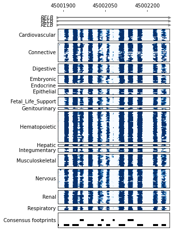
Plot gene annotations and heatmap

# We are grouping by biosample taxonomy
# level=1 is second level of multi-index
group_sizes=posteriors.groupby(level=1).size()
num_groups=group_sizes.shape[0]

# Code to draw figure
fig=plt.figure()
gs=gridspec.GridSpec(num_groups+2, 1, height_ratios=[0.1] + list(group_sizes/np.sum(group_sizes)) + [0.1])

# Plot gene track

# Gencode annotation
gencode_file_url = "https://resources.altius.org/~jvierstra/projects/footprinting.2020/annotations/"
gencode_file_url += "gencode.v25.chr_patch_hapl_scaff.basic.annotation.gff3.gz"

ax=fig.add_subplot(gs[0,:])
trk_genes = gencode_annotation_track(interval)
trk_genes.load_data(gencode_file_url)
trk_genes.render(ax)

ax.xaxis.set_visible(True)
ax.xaxis.set_ticks_position("top")

#
row=1
for group, df in posteriors.groupby(level=1):
    ax=fig.add_subplot(gs[row,:])
    ax.pcolormesh(1-np.exp(-df), cmap="Blues")
    ax.xaxis.set_visible(False)

    ax.yaxis.set_ticks([])
    ax.set_ylabel(group, rotation=0, ha="right", va="center")

    row+=1

#
ax=fig.add_subplot(gs[row,:])

fps_file_url="https://resources.altius.org/~jvierstra/projects/footprinting.2020/consensus.index/"
fps_file_url+="consensus_footprints_and_motifs_hg38.bed.gz"

trk_fps=segment_track(interval, edgecolor=None, facecolor="k")
trk_fps.load_data(fps_file_url)
trk_fps.render(ax)

ax.yaxis.set_visible(True)
ax.yaxis.set_ticks([])
ax.set_ylabel("Consensus footprints", rotation=0, ha="right", va="center")

fig.set_size_inches(4, 8)

previous

Emperical Bayes footprint detection

next

Footprint calling and plotting of a single DHS